After showing my previous post around at work, a colleague responded with this article in which the author compares the performance of a Java EE application running on Windows and on Linux. When running on Linux, the application exhibits the performance characteristics outlined in my post: at high utilisation, latency grows uncontrollably. What might be surprising however is that on Windows, latency doesn’t change much at all, even at high utilisation. Does this mean that the results we saw for \(M/M/1\) queues are wrong? Not quite! Whereas the Linux results show increased latency at high utilisation, the Windows results show an increased error count; at high utilisation Windows is simply dropping connections and kicking waiting customers out of the queue.
Recall from the discussion on \(M/M/1\) queues that we assumed the queue was of infinite size. No matter the load, there’s always space for a new customer in an \(M/M/1\) queue. The behaviour exhibited by the Windows system in the article isn’t that of an infinite queue, but instead that of a finite queue. At some limit - the precise details of which are irrelevant to this discussion - the queue gets full and customers are rejected.
What’s the latency like for a queue that has finite size? If the queue can reject customers, what’s the probability that a potential customer will be allowed in to the queue? Let’s answer these questions by looking at the \(M/M/1/K\) model.
An \(M/M/1/K\) queue behaves much like an \(M/M/1\), arrivals are a Poisson process, service times are exponentially-distributed and there is a single server. However, unlike \(M/M/1\) queues which allow an unbounded number of customers into the system at any time, \(M/M/1/K\) queues have an upper bound of \(K\) customers.
Steady-State Probabilities
All of the interesting calculations for \(M/M/1/K\) queues depend on the steady-state probabilities, that is, the probability \(p_{n}\) that there are \(n\) customers in the queue:
\[p_{n} = \begin{cases} \frac{(1 - \rho)\rho^{n}}{1 - \rho^{K + 1}} & (\rho \neq 1)\\ \frac{1}{K + 1} & (\rho = 1) \\ \end{cases}\]Where \(\rho = \lambda / \mu\), \(\lambda\) is the arrival rate and \(\mu\) is the service rate. Unlike the steady-state probabilities for \(M/M/1\) queues, the probabilities for \(M/M/1/K\) queues are defined for \(\rho \geq 1\) thanks to the limiting factor of \(k\).
Average Customers in the System
Using the steady-state probabilities we can now calculate the average number of customers in the system \(L\):
\[L = \sum_{n=0}^{K} n \cdot p_{n} \\\]We can plot the mean number of customers in the system as \(\rho\) increases and with \(K = 10\):
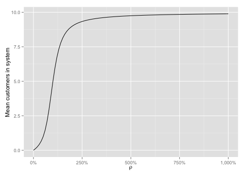
As we can see, no matter how large \(\rho\) gets, the number of customers in the system never exceeds the bound set by \(K\).
Calculating Average Latency
Now that we can calculate the average number of customers in the system for a given \(\rho\), we can use Little’s Law to calculate the mean latency. Recall from the discussion of \(M/M/1\) queues that Little’s Law relates the average number of customers in the system \(L\) to the average waiting time \(W\) and the arrival rate \(\lambda\):
\[L = \lambda W\]Which we can re-arrange to:
\[W = \frac{L}{\lambda}\]We might think that we can proceed from here to calculate the latency for one of our \(M/M/1/K\) queues, but first we must ask ourselves: is \(\lambda\) really a good measure of the arrival rate? Sure, \(\lambda\) is a good measure of the rate at which customers want to arrive in the system, but thanks to our limit \(K\), the effective arrival rate does not grow unbounded; \(\lambda\) is not a good measure of the number of arrivals that actually make it into the system. We’ll call this effective arrival rate \(\lambda_{eff}\).
We calculate \(\lambda_{eff}\) by realising that we will accept customers into the system if we’re not at the limit \(K\). Using our steady-state probabilities we have:
\[\lambda_{eff} = \lambda \cdot (1 - p_{K})\]That is, the effective arrival rate is the arrival rate multiplied by the probability that we are not at maximum capacity. We can now calculate latency using the effective arrival rate:
\[W = \frac{L}{\lambda_{eff}}\]Plotting the wait time of \(M/M/1\) and \(M/M/1/K\) graphs side-by-side as \(\lambda\) increases shows us how the limit \(K\) affects latencies at high \(\rho\). For these graphs \(\mu = 100\) and \(K = 10\):
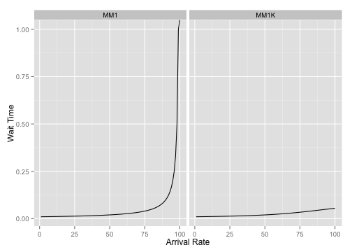
We can see how the latency profile of the \(M/M/1/K\) graph doesn’t have the same degenerate behaviour that the \(M/M/1\) queue has; the finite queue size prevents customers from seeing unbounded latencies.
Probability of Getting Rejected
If customers aren’t seeing unbounded latencies does that make finite queues some kind of panacea? Obviously not! As we know from the Windows vs. Linux benchmark that motivated this article, Windows traded unacceptable latencies for an increased error count. We can quantify this error count by calculating the probability of a customer getting rejected. We call this the loss probability \(p_{loss}\). It doesn’t take much thought to realise that the probability of getting rejected is simply \(p_{K}\), the probability that the queue is full:
\[p_{loss} = \begin{cases} \frac{(1 - \rho)\rho^{K}}{1 - \rho^{K + 1}} & (\rho \neq 1)\\ \frac{1}{K + 1} & (\rho = 1) \\ \end{cases}\]We can plot \(p_{loss}\) against \(\rho\) to see how the chance of seeing an error increases as \(\rho\) increases:
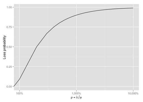
Here we can see that, as the arrival rate nears the service rate (\(\rho\) increases), the loss probability tends towards 100%. Note the log scale on the x-axis to get a real feel for the fact that even at \(\rho = 1000%\) the probability of loss still isn’t 100%.
A Note on Utilisation
In my previous post I referred to the quantity \(\rho\) as the utilisation of the queue. This was a little imprecise, because \(\rho\) is not a measure of utilisation for all queues. Let’s dig deeper to really understand what \(\rho\) and utilisation are measuring.
The ratio \(\rho = \lambda / \mu\) is a measure of traffic intensity. It tells us how much traffic is in the entire universe of our queue and how much processing capacity we have. Utilisation is a quantity that tells us how busy our system is. For \(M/M/1\) queues, which have no bound, \(\rho\) and utilisation are the same, because we’re never going to turn away a customer.
For \(M/M/1/K\) queues, \(\rho\) represents the intensity of traffic that we are seeing, but the utilisation tells us how much of that traffic is actually occupying the system. It should be obvious that we can measure utilisation as the probability that the system is not empty \(U = 1 - p_{0}\).
The relationship between \(\rho\) and \(U\) is easy to see with a plot:
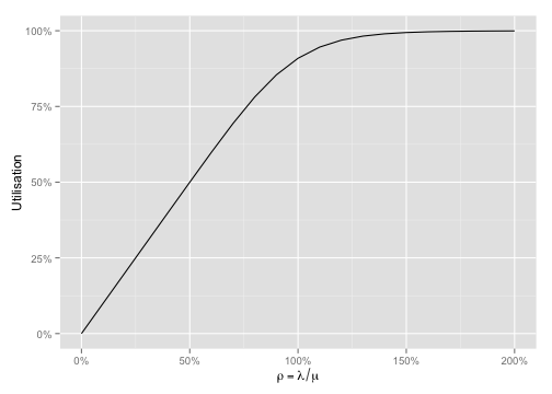
Notice how utilisation hits 100% after \(\rho\) passes 100% - this is the limiting factor \(K\) in action.
Conclusion
The benchmark that motivated this article showed that we can trade unbounded latency for an increase in rejected connections. While the Linux system behaved like an \(M/M/1\) queue, letting latencies grow but trying to serve every request, the Windows system behaved like an \(M/M/1/K\) queue, guaranteeing an acceptable latency for all requests that were accepted, but rejecting most requests when the system was heavily utilised.
The question remains: is it better to let latencies grow or should we reject some customers to ensure others get a better service? The answer to this question largely depends on the circumstances of your system, but it should be apparent that latencies get unacceptable quickly if your system is loaded and you’re not limiting the number of customers you serve. In my opinion, it’s better to preserve good service for a smaller number of customers rather than give bad service to all customers, which is what will happen as latency starts to degenerate under heavy load if your queue isn’t bounded.