In my previous post I presented the \(M/M/c\) queue as a model for multi-server architectures. As discussed at the end of that post, the \(M/M/c\) model has two main drawbacks: each server must have the same service rate, and there’s no mechanism for modelling the overhead of routing between servers. Modelling a multi-server system using a single queue - even a queue with multiple servers - ignores important real-world system characteristics. In this post, I’ll explain how we can arrange queues into networks that capture the cost of routing and allow for servers with different service rates.
Open Jackson Networks
We’re going to concern ourselves with a particular class of queue network called open Jackson networks. The ‘open’ in the name refers to the fact that customers arrive from outside the system much like the queues we’ve seen so far. In a closed Jackson network, there are no arrivals from the outside and customers never leave the system; in other words the amount of work in the system is constant.
The most interesting characteristic of Jackson networks is that they have a product form solution for the steady-state distribution. This is a rather grand way of saying that we can calculate the steady-state distribution of the network by treating each queue as if it were operating independently. For Jackson’s theorem to apply, all routing between queues in the network must be Markovian, that is routing of customers between nodes in the network is probabilistic.
At first glance, the requirement to route probabilistically might seem rather restrictive, but in reality it merely requires a small change in mindset. If our real world system routes traffic between \(n\) servers in a round-robin fashion, then our model can route between \(n\) queues with probability \(1/n\).
Modelling Load Balanced Servers
To get a better understanding for Jackson networks, let’s consider a concrete example of two servers operating behind a load balancer:
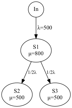
Here you can see that traffic arrives at the load balancer (\(s_{1}\)) from the outside with rate \(\lambda = 500\) and is then routed between each of the servers (\(s_{2}\) and \(s_{3}\)) with probability \(1/2\).
The probability that a customer leaves queue \(i\) and enters queue \(j\) is \(p_{ij}\). We use the index \(0\) to represent the outside world, so \(p_{0j}\) is the probability that a job enters queue \(j\) from the outside world and \(p_{j0}\) is the probability that a job leaves queue \(j\) for the outside world.
We can represent these routing probabilities as a matrix:
\[\begin{bmatrix} 0 & 1 & 0 & 0 \\ 0 & 0 & 1/2 & 1/2 \\ 1 & 0 & 0 & 0 \\ 1 & 0 & 0 & 0 \\ \end{bmatrix}\]We see from the matrix that \(p_{01}\), the probability that a job enters queue \(1\) from outside the system is \(1\) and the probability that jobs move from queue \(1\) to either queue \(2\) or queue \(3\) is \(1/2\).
Jackson’s theorem tells us that, provided we have Markovian routing, and that each queue has its own well-defined steady state, then the whole network has a well-defined steady-state distribution. Furthermore, the product form rule tells us the network’s steady-state distribution:
\[p(\mathbf{n}) = \prod_{i=1}^{J} p_{i}(n_{i})\]The important point here is that each queue must have a well-defined steady state. If not, then the product form rule does not apply. So then, how do we determine if each queue in a network has a well-defined steady state? For that we need to calculate the flow balance equations.
Flow Balance
The flow balance equations for a network with \(J\) queues is a set of \(J\) equations that we can solve to find the effective arrival rate \(\lambda_{i}\) at each queue \(i\).
Looking back at our matrix of routing probabilities, it should be clear that any queue can receive customers from the outside world, but also that customers can flow in cycles through the network. Nothing in the Jackson model requires that the network is acyclic. Thus the effective arrival rate for each queue must account for arrivals from outside and for arrivals from all other queues within the network.
More formally, the flow balance equations for a Jackson network with \(J\) nodes are:
\[\lambda_j = \lambda_{0j} + \sum_{i=1}^{J} \lambda_i \cdot p_{ij}\]Working through this we see that the effective arrival rate at each queue \(j\) is \(\lambda_j\), the sum of all arrivals from other queues, adjusted by the corresponding routing probability, plus the arrivals from outside the system.
Our sample network is a special case: a feed forward network. In a feed forward network, the network must be acyclic and customers cannot appear in the same queue more than once. Calculating flow balance for such networks is greatly simplified as we can see by working through the flow balance for each queue:
\[\begin{align} \lambda_1 &= \lambda \\ \lambda_2 &= 1/2 \lambda \\ \lambda_3 &= 1/2 \lambda \end{align}\]Recall from the discussion of \(M/M/1\) queues that the stability condition for \(M/M/1\) is \(\rho = \lambda / \mu < 1\). If this condition holds for each of our queues, then we know that our network has a steady-state distribution given by Jackson’s theorem. Using the service rates from the diagram above we can calculate \(\rho\) for each of our queues:
\[\begin{align} \rho_1 &= \lambda_1 / \mu_1 = 500 / 800 = 0.625 \\ \rho_2 &= \lambda_2 / \mu_2 = 250 / 500 = 0.5 \\ \rho_3 &= \lambda_3 / \mu_3 = 250 / 500 = 0.5 \end{align}\]Since \(\rho < 1\) for all our queues we know that each queue is stable and thus the network is stable.
Steady-State Probabilities
With the knowledge that our network has a well-defined steady state, we can apply Jackson’s theorem to calculate the steady-state probabilities for our network.
The steady-state probability for an \(M/M/1\) queue is \(p(n) = (1 - \rho) \rho^n\). Applying the product rule for Jackson network we get:
\[\begin{align} p(\mathbf{n}) &= (1 - \rho_1) (1 - \rho_2) (1 - \rho_3) \rho_1^{n_1} \rho_2^{n_2} \rho_3^{n_3} \\ &= 0.375 \cdot 0.5 \cdot 0.5 \cdot 0.625^{n_1} \cdot 0.5^{n_2} \cdot 0.5^{n_3} \\ &= 0.09375 \cdot 0.625^{n_1} \cdot 0.5^{n_2} \cdot 0.5^{n_3} \\ \end{align}\]Let’s now calculate the probability that we have two customers at each of the queues, that is, let’s calculate \(p(\langle 2, 2, 2 \rangle)\):
\[\begin{align} p(\langle 2, 2, 2 \rangle) &= 0.09375 \cdot 0.625^{n_1} \cdot 0.5^{n_2} \cdot 0.5^{n_3} \\ &\approx 0.0022888 \end{align}\]Latency of Queue Networks
As with the queue models we’ve seen so far, the steady-state probabilities are not that interesting on their own. Rather, the results that follow from these probabilities are what interest us. To determine the average latency for the network \(W_{net}\) recall Little’s Law:
\[L = \lambda W\]The mean number of customers \(L\) is equal to the arrival rate \(\lambda\) multiplied by the mean latency \(W\). We know the arrival rate for our network, so we if can calculate the mean number of customers in the network, the latency will follow. Since we are able to consider each queue in isolation after solving the flow balance equations, it’s enough to calculate the mean number of customers for each queue and then sum them:
\[L_{net} = \sum_{i=1}^{J}L_i = \sum_{i=1}^{J} \frac{\rho_i}{1 - \rho_i}\]For our network:
\[\begin{align} L_{net} &= \frac{\rho_1}{1 - \rho_1} + \frac{\rho_2}{1 - \rho_2} + \frac{\rho_3}{1 - \rho_3} \\ &= \frac{0.625}{0.375} + \frac{0.5}{0.5} + \frac{0.5}{0.5} \\ &\approx 3.6667 \end{align}\]With \(L_{net}\) in hand, we can now calculate the latency \(W_{net}\) for our network:
\[\begin{align} W_{net} &= \frac{L_{net}}{\lambda} \\ &\approx \frac{3.6667}{500} \\ &\approx 0.0073334 \end{align}\]Coarse-grained results such as average wait time and average occupancy gives us rough insight into our queue networks. We can gain better insight using simulation tools such as PDQ and SimJS. SimJS provides a drag-and-drop interface for designing queue networks and can simulate many hours of queue activity in a handful of minutes.
I plan to write about network simulation more in a later entry, but for now I recommend you try out SimJS.
Conclusion
Queue networks are a useful tool for modelling complex distributed applications. We gain the simplicity of Jackson networks provided we ensure Markovian routing throughout our model. If our network is free from cycles, calculating flow balance is simply a case of tracing traffic from the entrypoints of the network all the way through to the exit points.
When modelling your own systems using queue theory, prefer network models over \(M/M/c\) models. Networks afford the flexibility to model varying service rates across the servers in the network, and provide a means to model the overhead of traffic routing.